The synthetic control method

To motivate the use of the synthetic control method for quasiexperimental studies of injury control interventions, we can begin by considering its theoretical underpinnings using the potential outcomes framework.9

First, let us define the data requirements involved. To apply the method, we must have dataset containing repeated observations for  N units (eg, regions, countries, groups or individuals)  over T time periods (eg, months and years), commonly referred to as panel or time series cross-sectional data. Typically, the method is applied to aggregate data, which are readily available to injury epidemiologists through public health information systems (eg, CDC’s Wide-ranging Online Data for Epidemiologic Research (WONDER) database, which contains panel data for states and counties in the USA). The dataset must be balanced with respect to the temporal dimension, which means that an outcome variable  is observed for all units j over the same time periods  t (see appended data for an example).

Let  represent some intervention or natural experiment of interest coded as 1 for observations in the postintervention period in the treated unit and 0 otherwise. For a binary intervention, such as  , we can define two potential outcomes for each unit   j and time period t . Using the synthetic control method, our goal is to estimate the causal effect of an intervention on a single intervention unit, . The effect is defined as , where  is the observed potential outcome in the postintervention period  and is a an unobservable counterfactual state in which the unit was not exposed to the intervention. To estimate the effect,  , we must therefore attempt to quantify  using a set of concurrent control units from a so-called donor pool of untreated units . The question then becomes: how do we select our control units in such a way that they are most likely to represent ? And what if there is no such control in the data, or what if we are uncertain that we have found the optimal control unit?

Abadie and Gardeazabal2 provide a potential answer to these questions that exploit preintervention data and matching methods to avoid many of the pitfalls of classic quasiexperimental evaluation methods. The synthetic control method, which Abadie et al later chose to call it,3 is an extension of the difference-in-differences method (or controlled before–after study) that enables the analyst to automatically select and generate a control unit from a donor pool of potential controls. This is achieved through convex optimisation and weighting such that the synthetic control unit closely resembles the intervention unit in the preintervention period on the outcome variable and a set of user-specified covariates, by simultaneously minimising the difference in preintervention covariate composition and root mean squared prediction error (RMSPE) in the same period.

As such, the method is more likely to produce internally valid estimates as compared with a manual selection of controls (which is sensitive to user specification error or biased selection of control units). This is because it optimises the control selection by directly addressing the causal assumptions behind the difference-in-differences approach: the common trends assumption (ie, that both the treated and control groups must follow parallel paths on the outcome over time). Thus, the selection is mainly data driven and tailored towards causal inference theory. A major strength of the method is also that the control unit is a weighted average of all potential controls in the data. By also considering all possible weighted combinations of control units, we do not limit the search for the best control group to the states as they appear originally in the data (e.g. by simple omission or inclusion of certain states as control units), which should increase the chance of finding a valid counterfactual.

Specifically, with the goal of minimising the preintervention RMSPE, the synthetic control method obtains a set of weights  for each units in the donor pool, stored in a vector  that is constrained to be non-negative and sum to 1, the effect estimator

yields an unbiased estimate of the effect at time t under the assumption that the synthetic control sufficiently captures all unobserved time-varying confounding factors throughout the study period using the preintervention period as training data. As Abadie et al show in their mathematical proofs,3 the method will capture these factors if the synthetic control unit is accurately able to predict the preintervention evolution of the outcome in the treated unit, at least as the number of time points in the preperiod approach infinity. As a result, the risk of bias increases if the preintervention fit is poor or if the preperiod is too short (especially if the variance in the outcome variable is large). I will return to these points later in the discussion. For now, it is sufficient to note that we must also rely on the assumptions that there are no concurrent events specific to the intervention group in the postperiod that can explain the results and that there are no spillover effects into one or many of the groups in the donor pool, especially if these receive large weights. Thus, the method is not immune to bias, and it is up to the analyst to determine the sensitivity to such errors and, for example, remove invalid controls from the donor pool. Nonetheless, assuming the risk of bias from these violations is determined to be acceptable, we can proceed with the analysis.

As noted above, the optimal weights are estimated by minimising the RMSPE for the preintervention period, which measures the fit of the synthetic control unit. The RMSPE is given by

where  is the total number of time periods in the preintervention period (note that the RMSPE can be analogously defined for the postintervention period).10 We will use this measure to perform permutation tests below.

Application

To demonstrate the process, let us apply the method to a real case using publicly available injury data (the dataset and replication codes for Stata are available in the online appendix).

Results

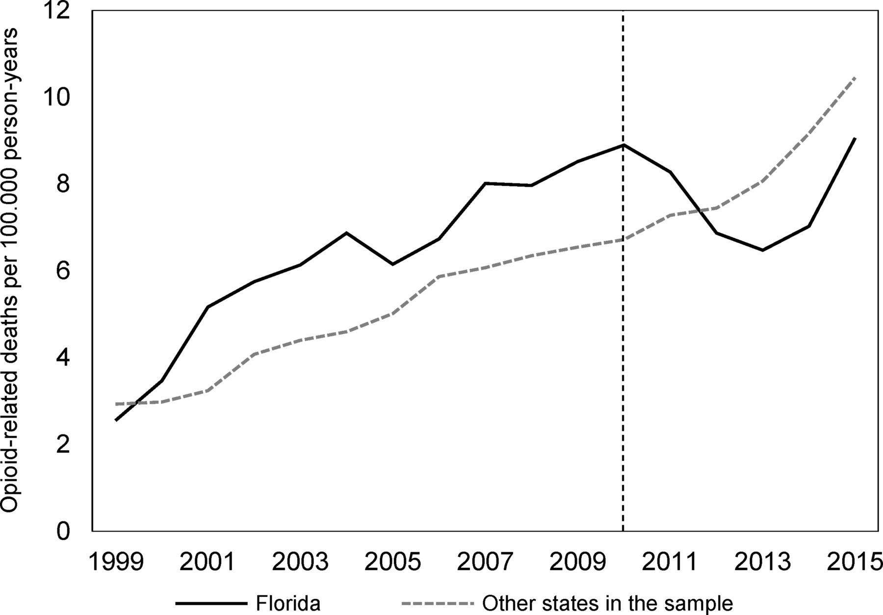
We begin by examining the raw data. Figure 1 compares the incidence of opioid-related deaths per 100.000 person-years in Florida to the remaining states in the donor pool (after removing states with gaps on the outcome). As we can see there, the overall sample of untreated states provides a poor counterfactual. We can clearly see an indication of an effect at the time of the intervention, but the information contained in figure 1 is not enough to quantify its shape or size.

• Download figure
• Open in new tab
• Download powerpoint

Figure 1

Trends in opioid-related deaths per 100.000 person-years in Florida and the unweighted donor pool (the vertical line indicates the start of the intervention period).

Let us move to the creation of the synthetic control unit. While Abadie et al argue that the major strength of the method is that it circumvents researcher specification error in the choice of the optimal control unit,3 we are still faced with the dilemma of specifying a vector of preintervention outcomes to match on. Ferman et al list a set of common choices that follow logical rules: (1) matching on the average of all preintervention outcomes, (2) matching on the entire range of preintervention outcomes (point-by-point), (3) matching on the first half, (4) matching on the first three-fourths, (5) matching on values from every odd year or (6) matching on even years.19 Since this choice might affect the results and lead to cherry picking, they suggest running all these analyses and choosing the model that minimises the preintervention RMSPE. One problem with this procedure is that (2) will almost invariantly minimise the RMSPE since the matching takes place on all years, and Kaul et al 20 warn against doing this if other covariates are included in the model since their variable weights will then automatically be set to zero (see below for an explanation of these weights, which are different from the unit weights discussed above). Since a set of covariates are included in the analysis, I select the model that minimises the RMSPE of the other options, which in this case is (6).

The resulting ‘synthetic Florida’ is a weighted average of the outcomes in Maine (46.1%), Pennsylvania (34.4%), Nevada (5.4%), Washington (5.3%), West Virginia (4.3%) and Oklahoma (3.4%). The entire unit weight matrix is presented in table 1. Figure 2 compares the synthetic control unit to the observed outcomes in Florida. As we can see there, the model fits the data well in the preperiod and indicates an effect in the expected direction in the postperiod. Results for the other specifications are displayed in online appendix figure A1 , where we can see that they also show similar effect estimates (note that the main result happens to be the most conservative of the options).

Supplementary file 2

[SP2.pdf]

View this table:

• View inline
• View popup

Table 1

Unit weights for the synthetic control unit for Florida

• Download figure
• Open in new tab
• Download powerpoint

Figure 2

Trends in opioid-related deaths per 100.000 person-years in Florida and the synthetic control unit (the vertical line indicates the start of the intervention period).

Table 2 compares the actual Florida to the synthetic control, as well as the unweighted donor pool, to probe their resemblance in the preintervention period. This analysis also confirms what figure 1 indicates, that is, that the unweighted donor pool provides a poor counterfactual, at least in terms of preintervention incidence rates and per capita GDP. However, synthetic Florida provides a better predictor balance on all predictors except for per capita personal income. Note that this does not necessarily mean that synthetic Florida is a biased counterfactual. Recall that the optimisation routine assigns variable weights based on the predictive power of each covariate (that, similar to the unit weights, also sum to one) and assigns lower weights to poor predictors so that they are given less importance in the matching process. These weights are displayed in the V-weights column in table 2, where we can see that the vector of preintervention outcomes are given considerably higher weight than the covariates. Of the covariates, per capita GDP is assigned the highest weight (0.048), which indicates that this variable has some predictive power, while the other two are assigned much smaller weights (0.005 and 0.004).

View this table:

• View inline
• View popup

Table 2

Preintervention predictor balance check between Florida, synthetic Florida and the unweighted donor pool

The time-varying effect estimate, which is calculated by taking the difference between the outcomes in Florida and the synthetic control unit, is displayed in figure 3. There we can see that the effect appears to be delayed by 2 years and has been gradually increasing in magnitude over time (in the short run). However, more postintervention data are needed to determine the long-run shape and magnitude of the effect. In 2015, the estimated effect was −6.19 opioid-related deaths per 100.000 person-years, which corresponds to a relative effect of −40.60%. Using population size estimates of Florida from the US Census Bureau to derive the number of opioid-related deaths prevented from 2010 to 2015, the estimates in  figure 3 suggest that the cumulative effect amounts to 3013 opioid overdose deaths prevented over the course of the postperiod.

• Download figure
• Open in new tab
• Download powerpoint

Figure 3

Dynamic effect estimates for the Florida post-2010 opioid overdose interventions on the incidence of opioid-related deaths per 100.000 person-years.

Inference procedures

While attempts have been made to derive sampling-based inference statistics for the synthetic control method, these methods are still under development.21 Arguing that sampling-based inference does not say anything about the validity of the results, Abadie et al 3 suggest instead using permutation tests in the form of placebo studies on untreated units. The logic behind these tests are that we can pretend that the intervention took place in another unit by running the same synthetic control procedure on other states to check if similar results manifest elsewhere as well, which would weaken the case for causality. It should be noted that by random error, or by the occurrence of other events that we are unware of, we are likely to find some effects in other states as well. However, if the estimate for Florida lies on the tail of the distribution of estimated effects, we obtain greater confidence in the results.

To avoid assigning an implausibly large weight to placebo studies with a poor fitting synthetic control unit, it is also important to account for the preintervention fit in these permutation tests, since we worry mainly about placebo studies that outperform the main analysis in terms of preintervention fit and effect size. To this end, Abadie et al suggest calculating the ratio between the postintervention and preintervention RMSPE for all placebo studies as well as the main analysis.3 From this, we can derive a pseudo P value by calculating the probability of finding a post/pre-RMSPE ratio greater than or equal to the ratio in Florida. It is worth noting that the use of the term P value is slightly misleading since it is based on permutation tests and therefore not comparable with a real P value (eg, with a sample size of 10 states, the minimum possible ‘P value’ will be 1/10=0.10). We must therefore be willing to rely on more arbitrary decision rules when running these tests.

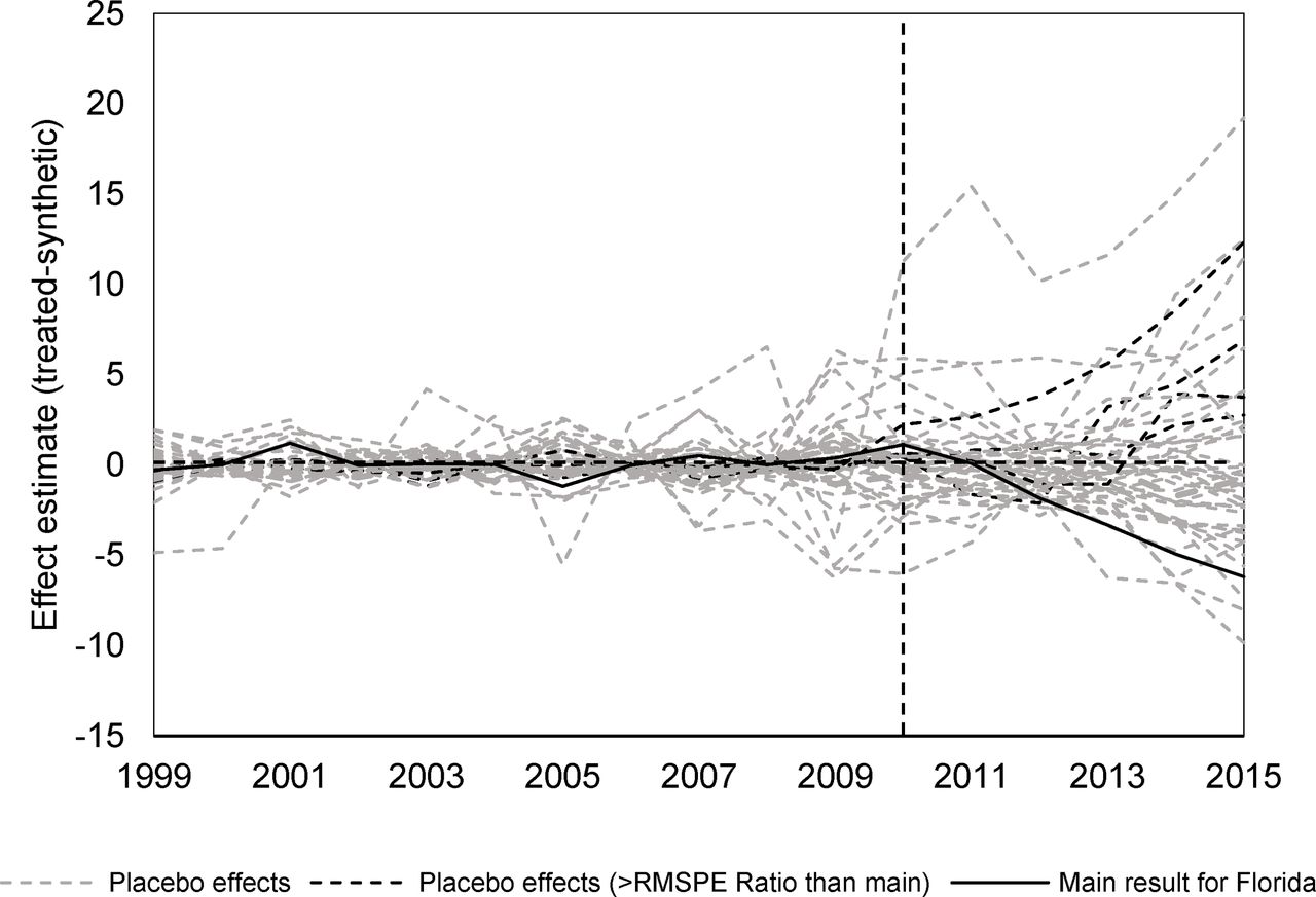
The inference procedures suggest a pseudo P value of 5/46=0.11, meaning that four placebo runs outperforms or equals the effect estimate for Florida when preintervention fit (RMSPE) is accounted for. These states are Connecticut, Indiana, Ohio and South Carolina, and the black dashed lines in figure 4 indicate their respective placebo results. The solid black line shows the result for Florida, and the grey dashed lines indicate placebo studies with poorer fit in the preperiod. As can be seen there, the placebo studies with good fit that outperformed Florida in terms of post/pre-RMSPE ratio all indicate effects in the opposite direction, which would yield a one-sided pseudo P value of 1/46=0.02. My assessment of this, in absence of a clear decision rule, is that the evidence for a causal effect of the Florida initiatives is strong.

• Download figure
• Open in new tab
• Download powerpoint

Figure 4

Dynamic effects for Florida compared to placebo studies on the 45 other states in the donor pool.

Sensitivity analysis

As a sensitivity analysis to ensure that the results are not produced as a consequence of single influential state in the synthetic control unit, I perform a leave-k-out analysis in which highly influential states are iteratively removed from the donor pool. Specifically, this is performed iteratively so that each iteration reduces the donor pool by one ( in the first iteration,  in the second and so on) and refits the synthetic control model using the restricted donor pool. For the first iteration, this means that we drop Maine from the donor pool based on the unit weights in table 1. After refitting the model, we find that Hawaii receives the highest unit weight and drop Hawaii (along with Maine) for the next iteration. This process can be repeated until only one state remains, but since we mainly care about synthetic controls with low prediction errors, I perform the iterations until the preintervention RMSPE is more than twice that of the main analysis (which yields 36 different synthetic controls including the main result). The results from this exercise are presented in figure 5 , where we can see that the synthetic control results are robust to the exclusion of influential states, which lends more credibility to the analysis. Notice also that the delay in the effect that we observed in the main analysis is not present in all iterations, which means that we are less certain about the shape and size of the effect during the first 2 years. The mean, median, 2.5th and 97.5th percentiles of these iterations are presented in online appendix table A1. The average estimate in 2015 was −4.55 deaths per 100.000 person-years (2.5th percentile: −1.24, 97.5th percentile: −7.92). The iterations suggest that the cumulative effect in terms of deaths prevented in the postperiod is 3705 (2.5th percentile: 1302, 97.5th percentile: 6412).

• Download figure
• Open in new tab
• Download powerpoint

Figure 5

Results from a leave-k-out analysis that iteratively reduces the donor pool by excluding the most influential state from the synthetic control unit until the pre-intervention prediction errors are twice as large as in the main analysis (n = 35 iterations).

Concluding discussion

I have demonstrated the potential value of the synthetic control method for measuring the population-level impact of injury prevention policies. It is especially useful for unique interventions and policy changes for which standard panel data approaches are inefficient. For the most part, it also provides a transparent and clear analysis that focuses on the causal assumptions of the difference-in-differences model, in ways that make it easy to assess the quality of the analysis by studying how well the synthetic control matches the pretreatment outcomes and covariates of the intervention unit. If the analysis is coupled with a transparent reporting of sensitivity analyses and placebo checks, we might stand to gain a greater level of confidence in estimates of the population-level impact of injury-related interventions compared with other quasiexperimental methods.

Yet, there are some caveats with the method that prospective analysts should be aware of. One is the lack of standardised decision rules for statistical inference (see, eg, Ferman and Pinto for a discussion of this issue).21 Even though Abadie et al argue that the synthetic control method forces the analyst to think about the causal assumptions of the model rather than sampling error,3 the optimisation routine still generates weights based on the observed outcomes in the preperiod. Hence, the bias of the synthetic control method will partly be a function of the random year-to-year variability of the data and is thus not free of this type of uncertainty. In a sense, the method based on the assumption that the random variability in large sample aggregate data is small to none,3 which limits its usage to panel data with small amounts of white noise. This may hold true for stable macroeconomic time series (such as GDP per capita), for which the method was developed, but in aggregate epidemiological datasets containing injury or disease incidence rates, the variance is also a function of the amount of events that occur.22 In practice, this means that it will likely be less useful for smaller regions, or uncommon types of injury events, since the low counts and high variance in such series will make it harder to find an optimal synthetic control unit due to matching on noise rather than the actual signal of the trend. In these cases, it may be better to use alternative methods.

An additional limitation that should be noted is that constraints are placed on the donor weights so that they are non-negative and must sum to one. According to Abadie et al,3 this choice was made to minimise the risk of extrapolation bias and overfitting,23 since allowing for any positive or negative weight to be associated with the donors will produce a perfect match in almost any case, but will likely result in poor out of sample predictions.24 Still, there are machine learning regularisation methods (lasso, ridge or elastic net regressions) that can be used to avoid this type of bias without imposing an explicit restriction on the weights, as discussed and tested by Doudchenko and Imbens,16 but these are not currently implemented in the Synth routines for Stata or R. In my experience, this constraint mainly becomes an issue if the intervention unit has the highest or lowest injury rate of all units before the intervention, meaning that there is no convex combination of donor units that can be interpolated to generate a synthetic control unit. If this is the case, the machine learning methods may be more appropriate if other quasiexperimental methods (eg, interrupted time series or difference-in-differences) appear infeasible.

Another limitation, which is more specific to my presentation of the method rather than its current state, is its limitation to a single intervention unit. This was at least the case with the original synthetic control method proposed by Abadie et al and used in their algorithms for Stata and R.3 10 However, Cavello et al and Kreif et al have examined extensions of the method to panel data with multiple intervention units and interventions with time-varying implementation dates (which can be useful to study, eg, the effects of US state laws with varying enactment years).25 26 Robbins et al 27 also consider extensions to multiple outcome measures in high-dimensional data settings, and Klößner and Pfieffer28 develop multivariate synthetic control models that allow for time series predictors. Xu29 also merges the synthetic control method with the interactive fixed effects framework in a recent paper, and Sills et al 30 discuss and implement a bootstrapping method to produce CIs for the counterfactual. As we can see, there are many developments not covered here, and prospective analysts will likely benefit from studying these recent advances as well.