Article Text

Abstract
Objective: To investigate the spatial patterning and possible contributors to the geographical distribution of suicide among 15–44- year-old men.
Design: Small-area analysis and mapping of geo-coded 1988–94 suicide mortality data and 1991 census data using random-effects smoothing.
Setting: 9265 electoral wards in England and Wales (mean population of men aged 15–44- years: about 1220).
Main results: Two main patterns emerged: (a) in all of the 10 most densely populated cities studied, suicide showed a “bull’s-eye” pattern with rates highest in the inner-city areas and, in some cases, low rates in the peripheries, and (b) suicide rates were high in coastal areas, particularly those in more remote regions. Possible indicators of social fragmentation, such as the proportion of single-person households in an area, were most strongly and consistently associated with rates of suicide in both urban and rural areas. Levels of unemployment and long-term illness accounted for some of the coastal patterning. Although characteristics of areas accounted for more than half of the observed variability, substantial between-area variability in rates remained unexplained.
Conclusions: The area characteristics investigated here did not fully account for the higher suicide rates observed in the most rural or remote areas. Alongside social and economic aspects, rural life itself may have an independent effect on the risk of suicide. A greater understanding of local geographies of suicide, and particularly the possible interactions between characteristics of people and their environments, might assist the design of prevention strategies that target those areas (and their characteristics) where risk is concentrated.
- SMR, standardised mortality ratio
Statistics from Altmetric.com
Each year, around 4500 deaths are given a suicide or an open (ie, undetermined whether accidentally or purposefully self-inflicted) verdict in England and Wales; nearly half of these deaths occur among men aged 15–44- years. Although suicide now ranks as a leading cause of death among young men, knowledge of its aetiology is limited. Notably, less than a quarter of the people in this group are in contact with specialist mental health services in the year before death.1 The UK government has recently put suicide on the public health agenda as an important contributor to area health inequalities.2 A key component to understanding these inequalities is a description of the geography of suicide—that is, whether observed variation (a) exceeds that expected by chance; (b) has a spatial pattern; (c) can be explained by known risk factors; and (d) any spatial patterning in unexplained variability can give additional clues about previously unidentified, or unaccounted for, risk factors. Identification of areas with high rates of suicide, and a better understanding of possible contributors, may allow the targeting of preventive efforts to those localities (and their characteristics) where risk is concentrated.
Although the age and sex distribution of suicide in England and Wales is well characterised, much less is known of its spatial patterning. Studies have generally focused on relatively large areas, such as local authorities,3 district counties4 or parliamentary constituencies5 (maximum 650 areas, average population aged ⩾15 years = ≥70 000), and commonly favoured simple statistical approaches that treat geographical areas as independent. Maps have commonly presented standardised mortality ratios (SMRs).6,7 When comparing small areas with varying population sizes, these can be particularly problematic. Areas with the smallest populations (usually the largest in size) produce the least reliable SMRs, as the variance of an SMR is inversely proportional to the expected number of events.8 Furthermore, maps based on small areas will have a substantial proportion of areas in which no events are observed, if the event is relatively rare.
Here, we use geographically appropriate methods to describe two inter-related aspects of the geography of suicide at a small-area level: (a) the magnitude and spatial patterning of suicide across wards in England and Wales and (b) the extent to which socioeconomic characteristics of areas explain the observed patterns. Our focus is on 15–44-year-old men; the age group that not only has the highest rates but also has experienced the most unfavourable trends in recent years against a backdrop of a decrease in rates among women and older men.9
METHODS
Mortality and population data
Suicide and undetermined deaths (International Classification of Diseases (ICD9) codes E950.0–E959.9 and E980.0–E989.9, excluding E988.8, predominantly used to accelerate registration of homicides) geocoded with the postcode of the last known address were obtained from the Office for National Statistics. Undetermined deaths were included in accordance with previous analyses, as research using psychiatric rather than legal criteria suggests that most deaths given an open verdict are suicide.10 To ensure sufficient events per area, analyses were based on the 7-year period 1988–94, centred around the census year (1991). Each postcode was assigned to the electoral ward it geographically corresponds with, and ward population figures in 5-year age bands from the 1991 census were used to produce population denominators.
Social, economic and health characteristics of areas
A total of 11 ward-based indicators of an area’s socioeconomic characteristics were obtained from the 1991 census: proportion of (1) single-person households; (2) households privately renting; (3) population mobility (ie, people with a different address the year before the census); (4) unmarried adult population; (5) households not owner occupied; (6) households without access to a car; (7) overcrowded households; (8) economically active unemployed people; (9) lone-parent households; (10) social class IV and V households; and (11) people with limiting long-term illness.
These indicators were previously shown to relate to area levels of suicide either as single indicators11–13 or as part of a composite score, such as the social fragmentation score and the Townsend deprivation index.5,14,15 The social fragmentation score (originally termed the “anomie score”15) is based on standardised levels (z scores) of variables (1)–(4) listed above. Similarly, variables (5)–(8) form the component parts of the Townsend deprivation index.
Rurality indices
We also categorised each ward on the basis of two rurality indices calculated using 1991 ward populations: (a) population density and (b) population potential as a measure of geographical remoteness. Low levels of population potential indicate remoteness from large centres of population, such as London, Birmingham and Manchester, even if the ward itself is highly populated (a simple illustration of its calculation has been presented elsewhere16).
Data analyses
Analyses were based on a total of 9265 electoral wards (mean male population aged 15–44- years, 1221). Wards in the business centre of London (n = 25), which are predominantly non-residential, were combined as a single area. To assess the robustness of the observed geographical patterning and ecological associations, all analyses were repeated at the parliamentary constituency level (569 areas, mean male population aged 15–44- years, about 20 000). Expected deaths in each area were calculated by multiplying national age-specific and sex-specific incidence rates (in 5-year age bands) in the 7-year period under investigation by the corresponding age-specific and sex-specific population-years at risk. These were then used to calculate indirect SMRs, defined as the ratio of observed to expected number of deaths, in each area.
Random-effects Poisson regression models were used to produce smoothed maps of suicide rates and investigate associations of suicide with area characteristics. These models allowed both for global between-area variability and also for the tendency of neighbouring areas to have similar rates (local variability). Smoothed rate ratios in each area were thus calculated as a weighted average of the observed area rate ratio, the global mean rate ratio and the rate ratio in neighbouring areas (taken here to be those areas sharing a border), with weights based on estimated levels of global and local variability.17–19 The less precise the estimated rate in an area is or the stronger the evidence that rates are homogeneous across the study region (ie, the smaller the variation beyond that expected by chance alone), the higher the amount of smoothing towards the national average. Alternatively, the more similar levels of suicide are in neighbouring areas (ie, the greater the evidence of spatial autocorrelation), the higher the amount of smoothing towards the local mean.
We also re-estimated smoothed rate ratios in each area after adjusting for the effect of area characteristics on suicide rates, to assess both the amount of variability in suicide rates explained by these characteristics and any spatial patterning in residual variability. Associations with each of the area characteristics were examined before and after controlling for the effect of all other characteristics in multivariable models. To assess the separate contribution of rurality in explaining the observed patterns, models (and maps) were repeated after excluding the rurality indicators and the levels of car ownership, as this variable may act as a proxy for geographical location. Models were also extended to allow the effects of the area characteristics to differ in rural and urban areas, defined, respectively, as those areas below or above median levels on either measure of rurality.
Model estimation
Models were fitted using Markov chain Monte Carlo methods20 in WinBUGS V.1.3 (Bayesian inference Using Gibbs Sampling). The built-in conditional autoregressive distribution was used to smooth rate ratios towards the local mean.21 Bayesian estimation requires specification of hierarchical probabilistic distributions for all random effects and their parameters. Vague distributions (ie, not favouring particular values) were chosen in all cases, and sensitivity analyses with different specifications were carried out to assess the effect of the original choices.22 Standard diagnostics were used to confirm successful convergence of the simulations (ie, using the built-in Gelman–Rubin statistic based on values of four chains running in parallel from overdispersed starting values),23 and model fit was assessed by calculating the deviance information criterion.24
Mapping
All maps were produced using the Arcview 3.2 geographical information system (developed by the Environmental Systems Research Institute, ESRI. www.esri.com). Rate ratios (and residual rate ratios) lower and higher than those close to the national average (rate ratios of 0.9–1.1) are presented in blue and orange (and varying lightness), respectively. Categories of rate ratios symmetrical on the logarithmic scale are presented—for example, areas where rates are half (<0.5) and double (>2.0) the national average represent up to fourfold difference in rates.
As wards are designed to be of similar population size for census purposes, several densely populated inner-city wards are much smaller in area size than elsewhere in the country. Patterns of suicide mortality in the top ten concentrations of such small-sized wards were displayed in more detail. These were (1) the Greater London area, (2) Birmingham, (3) Manchester, (4) Liverpool, (5) Sheffield, (6) Leeds, (7) Nottingham, (8) Newcastle, (9) Cardiff and (10) Bristol.
RESULTS
There were 15 821 suicides in men aged 15–44- years between 1988 and 1994. Of these, 111 deaths with missing (0.6%) or incorrect (0.1%) postcodes were excluded from the analyses. Table 1 summarises the geographical distribution of deaths, population denominators, rate ratios and levels of all area characteristics investigated. The mean number of men aged 15–44- years across areas was 1221 (90% range 237–3218). At least one death was recorded in 66% of all areas and at least two deaths in more than a quarter of them. Even after excluding the 5% least and most extreme rates, up to ninefold differences across areas with at least one death were observed (rate ratios 0.42 and 3.73). When smoothed towards the global (ie, national) and local (ie, in neighbouring areas) mean, up to fourfold differences remained (rate ratios 0.61 and 2.55).
Summary statistics of the distribution of the number, raw standardised mortality ratios and smoothed rate ratios of suicide and undetermined deaths in men aged 15–44- years in 1988–94, as well as population denominators (men aged 15–44- years) and area characteristics (all ages) from the 1991 census across electoral wards in England and Wales (n = 9265)
Figure 1a shows the geographical distribution of SMRs. Most inner-city areas exhibited high rates. High rates were also found in several rural areas. However, with several areas recording no deaths, unequal sizes of wards in rural and urban areas, differing population structure and uncertainty associated with each of the estimates (particularly in rural areas), any inference about spatial patterning from a map of SMRs was difficult.
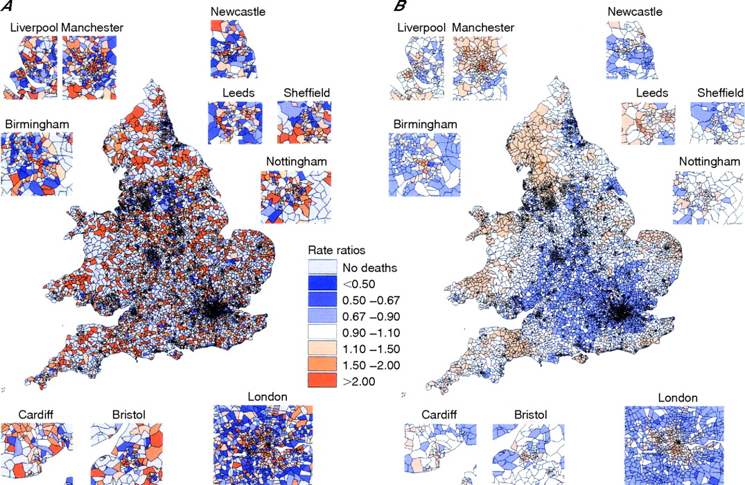
(A) Unsmoothed map of standardised mortality ratios (SMRs) of suicide in men aged 15–44- years across wards in England and Wales, 1988–94. Crude SMRs are shown for the incidence of suicide in men aged 15–44- years across wards (n = 9265) in England and Wales. As each SMR is estimated independently, the low numbers of events per ward means that there is substantial sampling variation, which makes the map difficult to interpret. Note that in 34% of all wards (shown in light grey) no deaths were recorded. (B) Globally and locally smoothed map of suicide in men aged 15–44 years across wards in England and Wales, 1988–94. The rate ratios shown were smoothed using a Bayesian hierarchical model incorporating both unstructured and spatially structured random effects. The smoothed rate in each ward is a weighted average of the observed (crude) rate, the global mean rate for all wards in England and Wales, and the local mean rate in neighbouring areas (taken here to be those areas sharing a border). Weights are based on estimated levels of global and local variability.
Figure 1b shows the smoothed map of suicide accounting for global and local variability. Unlike the “raw” map of SMRs, this displayed clear evidence of spatial patterning. Most inner-city areas retained their high rates; in Manchester, rates were more than double the national average. In the 10 cities investigated in more detail, a “bull’s-eye” pattern was observed with high rates in inner parts of cities and average, or in some cases below average, rates in their peripheries. These patterns were particularly clear in London, Manchester and Birmingham where rates differed by more than twofold from the centre to the outskirts. Similar differences where observed even when maps were only globally smoothed.
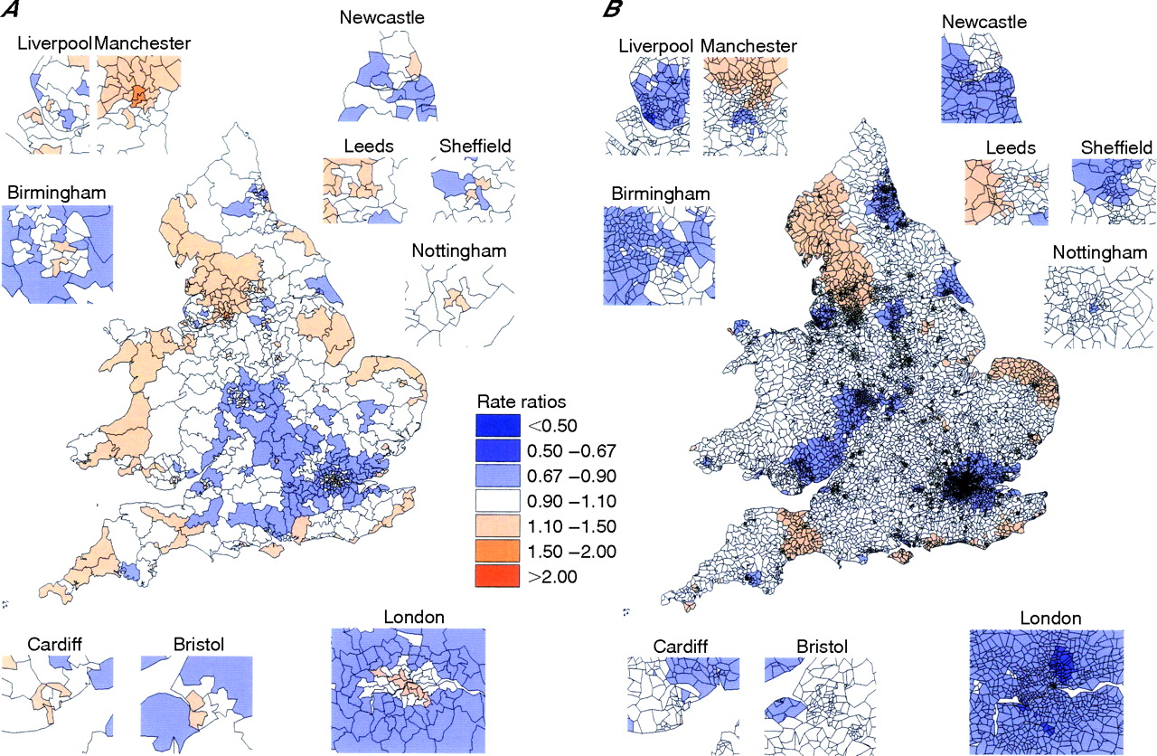
Also striking were the high rates observed in remote and coastal areas. Although particularly apparent on the west coast—for example, Wales (the broad peninsula on the west) and Cornwall (the south western tip of England)— smaller concentrations were also seen on the east and south coasts. Low rates seemed to concentrate in central parts of the country. Patterns seen in the smoothed map were replicated at the lower geographical resolution of constituencies (fig 2a). With an average population of 15–44-year-old-men of about 20 000 and the number of suicide deaths ranging from 9 to 75, this geographical level is not as prone to small number variation.
(A) Constituency-level globally and locally smoothed map of suicide in men aged 15–44 years in England and Wales, 1988–94. Smoothed estimates of suicide rate ratios are shown across constituencies (n = 569) in England and Wales. These were also derived using a Bayesian hierarchical model incorporating both unstructured and spatially structured random effects. The figure is displayed to assess the robustness of the observed patterns to the level of geographical resolution. (B) Residual rate ratios after controlling for all area characteristics excluding the rurality indicators. Smoothed estimates of the residual suicide rate ratios in each ward are shown after accounting for the association between area levels of suicide and their socioeconomic characteristics. Note that the rate ratios shown in the figure were estimated using models that excluded the otherwise substantial contribution of the rurality indicators—that is, population potential and population density.
Table 2 shows rate ratios of suicide associated with 1 standard deviation increase in levels of each of the area characteristics before and after controlling for the effect of all others. Increases in all socioeconomic characteristics investigated were, to some extent, associated with increases in suicide rates. However, after controlling for the effect of all characteristics, associations with the proportion of single-person or lone-parent households and unmarried people appeared the strongest. Associations with both measures of rurality were also particularly strong in multivariable models, with suicide rates increasing the lower the levels of either population density (indicating rurality) or population potential (indicating remoteness). After excluding the rurality indicators (or proxy measures such as levels of car ownership) to assess the separate contribution of socioeconomic characteristics of areas in explaining the observed patterns, over half of the variability was explained by socioeconomic area differences; yet, some twofold differences in rates remained unexplained.
Rate ratios (and 95% CrI*) of suicide in men aged 15–44 years associated with 1 SD increase in levels of each of the area characteristics in multivariable models controlling for the effect of all other single indicators and adjusting for spatial autocorrelation in the residual variability
Figure 2b shows geographical patterns of suicide not explained by differences in socioeconomic characteristics of areas. With the possible exception of Manchester, high rates in most urban areas were explained by the factors investigated. In fact, in several places (eg, London, Birmingham and Newcastle) rates even higher than those observed were expected based on levels of the area characteristics in these areas (as indicated by below-average rate ratios after accounting for area characteristics). Conversely, although the factors investigated partially accounted for the high rates in rural and remote parts of the country, some of the coastal patterning remained unexplained. Note that to highlight areas where socioeconomic characteristics of areas do not seem to explain some of the clusters of high rates of suicide, particularly along the coast, this map of residuals excludes the (otherwise substantial) contribution of the rurality indicators in explaining the observed patterns.
Evidence suggested that some factors may influence suicide rates differentially in different parts of the country. Levels of socioeconomic deprivation seemed more strongly associated with rates in urban than in rural areas. Conversely, for proportions of single-person households and unmarried populations, there was evidence that associations were stronger in the most remote parts of the country (p values for differential effects below and above median levels of population potential <0.01). Assessment of the separate contribution of each factor in explaining the coastal clusters suggested that the proportion of single-person households was possibly the single factor most consistently associated with patterns along much of the coast. However, other factors were important locally. For example, levels of unemployment and limiting long-term illness specifically accounted for some of the high rates observed in the west (eg, much of Wales and Cornwall). With the exception of the rurality indicators, no single factor, or even all put together (as presented here), seemed to fully explain some of the clusters on the northwest and east coasts.
DISCUSSION
Main findings
Area differences in suicide were greater than expected due to random variation alone. There were concentrations of high rates in inner cities and in several rural areas, particularly in remote or coastal regions. Nationally, indicators of social fragmentation, such as area proportions of single-person households and unmarried populations, were most consistently associated with rates of suicide in both urban and rural areas. Although rates of unemployment and long-term illness accounted for some of the tendency for increased rates in coastal areas, such patterns were not fully explained by any of the factors investigated here.
Limitations
Associations seen at an area level do not necessarily imply that such factors are associated with a person’s risk of suicide. However, the design and purpose of the study is to investigate possible contributors to the geographical patterning of suicide. Furthermore, the exposures we investigated were not age specific or sex specific. These indicators were, however, used to describe the overall social and economic characteristics of an area.
Geographical patterning
To date, the vast majority of area-based studies of suicide have focused on either large areas likely to mask important area variation across smaller communities,4,5 or smaller areas restricted to single regions25 or cities.14,15,26 Only a limited number have displayed the extent to which suicide varies geographically on a map6,7,27 and, with the exception of a series of studies in London,15,28 none has investigated possible contributors to these patterns.
Here, we improve on an earlier study of ward-level associations between socioeconomic area characteristics and levels of suicide13 to map the geographical variation in suicide at a finer level of geographical scale than previously used nationally in Britain, or elsewhere. We showed not only that the observed geographical variation in suicide is greater than expected due to random variation alone but also that neighbouring areas tend to exhibit similar levels of suicide.
Two of the more prominent features were the high rates in (a) inner-city and (b) coastal areas. As early as 1928, spot maps of suicide deaths in the city of Seattle suggested that suicide tends to be higher in central areas of the city and lower in the margins—“bull’s-eye” pattern.29 Patterns such as those observed here have been documented since then in the case of many cities—for example, Sydney,30 Edinburgh31 and more recently London.15,28 Inner-city areas tend to have higher levels of psychiatric morbidity32; however, the extent to which these patterns (observed to some extent in most big cities) reflect the effects of inner-city deprived environments on the mental health of their population is not known. Although some studies of suicide in Britain have reported high rates in some areas characterised as “coastal”, “resort” or “retirement”,6 the extent of the coastal patterning seen here has not been previously documented.
When locally smoothed, area estimates depend on the area’s number of neighbours; in fact, the variance of each area’s estimate is inversely proportional to its number of neighbours. As areas at the fringe of the country naturally tend to have fewer neighbours (commonly referred to in the literature as “edge effects”33), their rate ratios are estimated with higher variability. We have not explicitly adjusted for such possible “edge effects”. However, differences in the number of neighbours are not substantial: in the 25% most remote areas as indexed by population potential (ie, areas in the periphery of the country), the mean number of neighbouring wards was 5.3 (median 5, 90% range 2–9) as opposed to 5.7 (median 5, 90% range 3–9) in the rest of the country. Observed concentrations of coastal clusters extended inland, were apparent at both levels of geography and were also seen in other age and sex groups not presented here. Most importantly, the models presented here included both spatially structured (ie, smoothing towards the local mean likely to be affected by number of neighbours) and spatially unstructured effects (ie, smoothing towards the global mean). At least in the constituency-level analyses, high rates in coastal areas were also noticeable in maps where rate ratios were smoothed only towards the global mean (not presented here).
It was recently shown that the most adverse trends in suicide rates among young adults in recent years have occurred in the most rural or remote areas.16 Suicide in farmers—an occupational group in rural areas at increased risk of suicide and with easy access to particularly lethal suicide methods such as firearms—might contribute to some extent to the patterns observed in rural areas. Evidence, however, suggests that not only does the geographical distribution of suicide in farmers differ from that of the general population but also that, unlike the general population, rates in farmers declined between 1981 and 1993.34 Rather than the effect of a particular group, these patterns might reflect a more general rural disadvantage in terms of accessibility and utilisation of services, patterns of help-seeking behaviour, out-migration, stigmatisation of marital or mental health problems, or the seasonal nature of employment and social activities.
Area characteristics
There is little evidence regarding the appropriate scale for investigating contextual influences on a population’s mental health. With largely arbitrary boundaries, wards may have little relevance to true environmental influences on their populations, or indeed to people’s perceptions of their community. Although large enough to ensure that a reasonable proportion record some deaths, the wards are generally small enough to cover areas homogeneous in terms of their characteristics. Consistent with growing evidence from both Britain5 and abroad,35 our findings confirm that even at a small-area level, indicators of social fragmentation are important predictors of an area’s levels of suicide, independent of levels of deprivation.
The area characteristics investigated here did not fully account for the high rates observed in the most rural or remote areas. Factors not accounted for here (such as levels of alcohol consumption36 owing to lack of reliable area-level data) or the possible inability of measures of deprivation to adequately capture true levels of economic hardship in rural areas might further explain some of these patterns. Nevertheless, rural living itself may have an independent effect on the mental health of young adults, or exacerbate the effect of societal changes in some features, such as marital breakdown, traditionally not as common-part of rural as city life.
In contrast with previous ecological studies that generally find no37 or even inverse associations,4 this study found a positive (although relatively weak) association between levels of suicide and unemployment in young men, even after controlling for the effects of all other factors. This was observed only in models adjusting for spatial autocorrelation in the residual variability (such as those presented here). This is in keeping with recent findings of the increasing importance of levels of socioeconomic deprivation, and unemployment in particular, in explaining area differences in suicide among young men.38
Research and policy implications
Area differences in suicide mortality may reflect: (i) the aggregate risk of a concentration of people at high risk (compositional effects) and (ii) area influences of economic, social and cultural aspects of an area on a population’s mental health (contextual effects). As the concept of social capital has increased in popularity in recent years, so has interest in the extent to which area health inequalities are a product of “true” area effects.39 Most of the evidence on whether, and the extent to which, the place where people live matters comes from studies with a multilevel design. Independent effects on area levels of health have now been reported for a range of health outcomes.40 For mental health, however, the evidence is not as clear. To date, several studies have found no or only modest area effects,41–43 whereas others have reported contextual influences of area characteristics such as levels of socioeconomic disadvantage or residential mobility on mental health44,45 and suicide46,47 over and above the aggregate risk of their populations. Administrative definitions of areas might not coincide with people’s definitions, let alone perceptions, of their local community or neighbourhood. Furthermore, socioeconomic and cultural contextual influences might not necessarily be restricted to the area of residence. Both might limit our understanding of contextual influences on mental health.48
Importantly, the distinction between composition and context is not always straightforward. Explaining an area’s suicide rate as simply the result of its high-risk population (a purely compositional effect) risks ignoring what helps create compositional effects in the first place. Compositional effects can also arise from an inward drift of people at increased risk (similarly those at low risk may drift out) in search of certain features,49 such as higher tolerance, anonymity and availability of low-cost housing or hostels for the mentally ill, that such areas have to offer. Similarly, certain aspects of an area could have a direct effect on the likelihood of developing mental illness, or simply offer low levels of social support for the mentally ill.45 Aspects of an area—for example, the built environment, parks and local shops, activities of local community groups and networks may encourage (or discourage) educational and work aspirations and promote (or inhibit) social ties and support.50,51 There is, however, a relative lack of routinely available measures with national coverage that are truly contextual in nature—that is, that describe characteristics of the area where people live rather than their demographic composition.52
What is already known about this topic
-
There is wide geographical variation in the incidence of suicide internationally and across areas in Britain. However, the spatial patterning of suicide in Britain is not well explored.
-
Area socioeconomic characteristics, particularly indicators of social fragmentation, account for some of this variation but associations with known person-based risk factors, such as unemployment, are less clear.
What this paper adds
-
Rates of suicide in 15–44 year-old men are high in inner cities but are largely explained by the socioeconomic characteristics of these areas.
-
High rates of suicide also seem to concentrate in coastal regions, particularly those remote from large centres of population.
-
High levels of single-person households, unemployment and limiting long-term illness partly explain some of the observed coastal patterns.
Policy implications
Area-based suicide reduction strategies might benefit from targeting inner-city and remote coastal areas. However, a better understanding of local geographies is needed, in particular explanations for the heightened risk in coastal areas.
Suicide prevention strategies in many nations, including Britain, focus on primary or secondary healthcare prevention and access to lethal means. Policies that target only people may be unsuccessful if the general context in which health inequalities occur remained unchanged.53 Policies that might deal with such contexts include initiatives that aim to increase the social welfare and enhance residents’ satisfaction with their areas. Creating local employment opportunities may be particularly important in more rural or remote parts of the country. A greater understanding of local geographies of suicide, particularly possible cross-level interactions between characteristics of people and their environments, may inform appropriate reduction strategies (particularly where action is, or can be, taken at the local level) that target those areas and their particular characteristics where risk is concentrated.
Acknowledgments
We thank the Office for National Statistics, and Claire Griffiths in particular, for providing us with the mortality data; Danny Dorling (University of Sheffield) for all the socioeconomic, geographical-related and mapping-related data—for example, ward boundaries polygon files and postcode look-up files; and Peter Congdon, Tony Ades, Lesley Wood and Ben Wheeler for helpful discussions.
REFERENCES
Footnotes
-
Competing interests: None.
-
This study forms part of an original proposal put together by DG, JACS and NM for NM’s PhD, funded jointly by the University of Bristol and the Overseas Research Students (ORS) Award Scheme during which DG and JACS were NM’s PhD supervisors (2000–4). DG and NM collected the data. All analyses were performed by NM. JACS provided statistical advice. Maps appear in NM’s unpublished PhD thesis as part of a complete Atlas of suicide mortality and its socio-economic determinants in England & Wales. NM wrote the first draft of this paper. All authors contributed towards the final version.
Linked Articles
- In this issue